How to give title to your top journal science article
I was interested in web scraping and text/sentinel analysis with R and thought for a practice I can check what are the most commonly used words and phrases in a scientific top journal, like Nature or Science. Since these are general science journals, I would not expect any scientific field can take the lead, but let’s see.
First we need to access their page and see how their archive is built. If we can get some information where and how they store the issues and article titles, we can start with the rvest package. Let’s see the case of Nature.
Here I made a function to access any Volume - Issue pair on the page http://www.nature.com/nature/journal/vXXX/nYYYY/index.html where XXX is the volume (v) and YYYY is the issue (n). Luckily they store these in a consistent way, so we can easily get the titles from the #research tag’s hgroup html attributes. Firs let’s access the website with read_html(), then we can extract tags with html_nodes(). To transform this to a character vector, we use html_text() and save all these in a tibble. The last issue is v = 543 n = 7645, we can test with these.
library(tidyverse)
library(rvest)

nature_articles <- function(v, n) {
  read_html(paste("http://www.nature.com/nature/journal/v", v, "/n", n, "/index.html", sep="")) %>%
    html_nodes("#research") %>%
    html_nodes("hgroup") %>%
    html_text() %>%
    as_tibble %>%
    return()
}

nature_articles(v = 543, n = 7645)
## # A tibble: 28 x 1
## value
## <chr>
## 1 Astrophysics: Distant galaxies lack dark matter
## 2 Biomedicine: An improved gel for detached retinas
## 3 Physiology: Bone-derived hormone suppresses appetite
## 4 50 & 100 Years Ago
## 5 Biogeochemistry: A plan for efficient use of nitrogen fertilizers
## 6 Ecology: Coral crisis captured
## 7 Cell biology: Sort and destroy
## 8 Applied physics: 3D imaging for microchips
## 9 Molecular biology: A hidden competitive advantage of disorder
## 10 Mineral supply for sustainable development requires resource governance
## # ... with 18 more rowsThat’s great, we can get one issue’s titles, but we need years of articles, which means hundreds -if not thousands- of issues. First of all we need the correct volume-issue numbers and hopefully the corresponding publishing dates also. Nature in this case also provide a nice solutions, an archive website, http://www.nature.com/nature/archive/ where we can collect the necessary information. First of all let’s say we want to check the titles from 2015 and 2016. In this case our website URL modifies to http://www.nature.com/nature/archive/?years=2016-2015. I hope you get the pattern, because we will dynamically change this part depending what years we need. Other parts are very similar to the previous.
years = c(2012:2016)

read_html(paste("http://www.nature.com/nature/archive/?year=", paste(years, collapse="-"), sep="")) %>%
  html_nodes("dd") %>%
  html_text() -> issues

head(issues, 12)
## [1] "22 December 2016" "540" "7634"
## [4] "S97-S113" "22 December 2016" "540"
## [7] "7634" "486-614" "15 December 2016"
## [10] "540" "7633" "318-476"Great! Almost. OK, there are 2 problems: 2 unnecessary information is joint at the and (ISSN and EISSN numbers), we should remove them.
issues <- issues[seq_len(length(issues)-2)]The other one is the fact it is a character vector, not a data frame. If you look closely, very closely, you will figure out the 1st element is a date, then the issue, volume, finally the page numbers. This last one we do not need, so we will just discard, but the others still in a nice order we can use to arrange them into a tibble. Also there are some supplementary pages (SX-SY), those are generally replicated lines without the page numbers, so we will just extract the unique() lines. Then we need to filter special issues, which happened just a few times, but always got the S1 issue label.
n_issues <- tibble(
  date = parse_date(issues[c(T,F,F,F)], format = "%d %B %Y"),
  v = parse_number(issues[c(F,T,F,F)]),
  n = parse_number(issues[c(F,F,T,F)])
) %>%
  unique() %>%
  filter(n != 1)

n_issues
## # A tibble: 256 x 3
## date v n
## <date> <dbl> <dbl>
## 1 2016-12-22 540 7634
## 2 2016-12-15 540 7633
## 3 2016-12-08 540 7632
## 4 2016-12-01 540 7631
## 5 2016-11-24 539 7630
## 6 2016-11-17 539 7629
## 7 2016-11-10 539 7628
## 8 2016-11-03 539 7627
## 9 2016-10-27 538 7626
## 10 2016-10-20 538 7625
## # ... with 246 more rowsNow we have a data frame with one issue per line. To extract all the titles we will preserve this format and will use the magical list columns in tibble. To create the new column just use casually the mutate() function from the dplyr pkg. To perform our nature_articles() function on every line, we will use the map2() function from the purrr package, since we have two inputs to this function.
n_issues %>%
  mutate(
    titles = map2(
      v,
      n,
      nature_articles
      )
    ) -> all_title
all_title %>%
filter(lubridate::year(date) > 2011)## # A tibble: 6,498 x 4
## date v n
## <date> <dbl> <dbl>
## 1 2012-12-20 492 7429
## 2 2012-12-20 492 7429
## 3 2012-12-20 492 7429
## 4 2012-12-20 492 7429
## 5 2012-12-20 492 7429
## 6 2012-12-20 492 7429
## 7 2012-12-20 492 7429
## 8 2012-12-20 492 7429
## 9 2012-12-20 492 7429
## 10 2012-12-20 492 7429
## # ... with 6,488 more rows, and 1 more variables: value <chr>HTML error 503 if you want to collect a lot of data at once. Simply the website recognize your action as a bot or just cannot handle this many request. You can get a better chance if you put Sys.sleep() with some random values in the function or randomly change the user agent with curl::curl(). Check this and similar issues for more info.Now we have the necessary data, so let’s work on it. First we have to unnest() our data frame to have one title per line (or work with an already unnested data). Then tear them down to words and delete all the punctuation and case issues. For this the tidytext package’s unnest_token() function comes really handy.
Oh. And let me work from here with the data from 1998-2017.
library(tidytext)

all_title %>%
  unnest_tokens(word, value) -> all_words
Now we can count the words and see the most frequent ones are …
all_words %>%
  count(word, sort = TRUE)
## # A tibble: 28,943 x 2
## word nn
## <chr> <int>
## 1 of 13961
## 2 the 12917
## 3 in 10037
## 4 a 7252
## 5 and 6685
## 6 to 4629
## 7 for 4257
## 8 by 2676
## 9 on 2329
## 10 from 1825
## # ... with 28,933 more rows… not those we want. “of”, “the”, “in” and so on. These are called “stop words”. To remove them we can use the tidytext:stop_words data and dplyr::anti_join().
all_words %>%
  anti_join(stop_words, by = "word") %>%
  count(word, sort = TRUE)
## # A tibble: 28,358 x 2
## word nn
## <chr> <int>
## 1 science 1735
## 2 cell 1424
## 3 biology 1192
## 4 cells 985
## 5 human 953
## 6 research 878
## 7 protein 804
## 8 ago 758
## 9 structure 739
## 10 dna 726
## # ... with 28,348 more rowsNow we are getting very close what we need (or now we think we need). Here already in the first two lines you can see the problem. “cell” and “cells” are independent entries. If we want to remove every modifications from a word, that is called “stemming”, since we will get the “stem” of the word. In the “cell”, “cells” case of course “cell”. There are several methods and packages, like SnowballC, hunspell or tm. Here I am using SnowballC::wordStem().
library(SnowballC)

all_words %>%
  anti_join(stop_words, by = "word") %>%
  mutate(word = word %>% SnowballC::wordStem()) %>%
  count(word, sort = TRUE) -> word_count

word_count
## # A tibble: 20,363 x 2
## word nn
## <chr> <int>
## 1 cell 2409
## 2 scienc 1794
## 3 structur 1285
## 4 biologi 1192
## 5 research 1065
## 6 human 1064
## 7 protein 1029
## 8 genom 952
## 9 gene 850
## 10 activ 822
## # ... with 20,353 more rowsYou may ask why there are such strange words as “structur” and “biologi” instead of “structure” and “biology”. This is the result of stemming. “structure”, “structural”, “unstructured” and so on has the common stem “structur”.
For a fancy graph, let’s use the wordcloud2 package.
library(wordcloud2)

word_count %>%
  wordcloud2(backgroundColor = "black", color = 'random-light', shape = 'circle', gridSize = 6)
And in a little more usual form:
word_count %>%
  arrange(nn %>% desc()) %>%
  head(10) %>%
  ggplot(aes(x = reorder(word, -nn), y = nn)) +
  geom_bar(stat = "identity")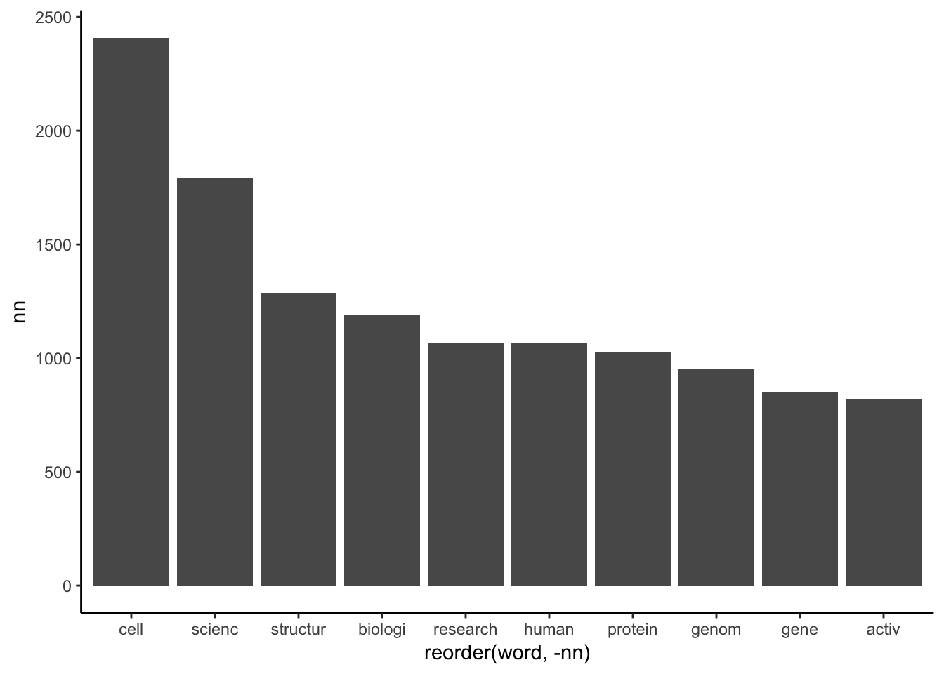
It is already really interesting. We can see, in the past 19 years the word “cell” was the most popular, exactly 2409 times popped up in Nature article titles. “Structure”, “cancer”, “biology”, “gene”, “genome”, “protein” and so are mainly life science related terms. It looks like Nature is a bit biology-biased or just biologists produce much higher amount of data and publications.
The world “cell” can be in many context, let’s find out in which context they appear the most (I bet stem cell and single cell RNA-seq are the most abundant, let’s take your bet, too). We can apply unnest_tokens() with token = "ngrams", n = 2 arguments to pick up 2-word phrases (2-grams) and in similar way as before we can count them.
all_title %>%
  unnest_tokens(word, value, token="ngrams", n = 2) %>%
  filter( stringr::str_detect(string = .$word, pattern = "[C|c]ell[s]*") == TRUE)  %>%
  count(word, sort = TRUE)
Indeed “stem cell(s)” was the most abundant, but “cell rna” was less usual (only 6 times), even then solar cells (12 times), probably because these terms just became popular and single cell sequencing is available from the last few years only. “single cell” was occuring 24 times (as “single cell activity”, “single cell division” and so on next to “single cell rna-seq”). Let’s have a look on the articles with “single cell” in the title.
all_title %>%
  filter( stringr::str_detect(.$value,
                              pattern = "[S|s]ingle([:graph:]|[:space:]){0,1}[C|c]ell")) %>%
  select(date, value)
## # A tibble: 30 x 2
## date
## <date>
## 1 2003-08-07
## 2 2005-07-21
## 3 2006-06-15
## 4 2007-06-28
## 5 2007-04-26
## 6 2009-02-12
## 7 2012-11-08
## 8 2012-07-05
## 9 2013-10-03
## 10 2013-08-29
## # ... with 20 more rows, and 1 more variables: value <chr>Interestingly the first article with “single cell” in the title just appeared in 2003 and after that only once in 2005, and once in 2006. Only from 2012 it became as popular to have some article in every year with the title containing this term.
Also let’s have a look on every 2-grams. Here I also separate the 2 words first to remove every stop word containing lines and stem them. Also “science” appears so many times due to article type headers, like “Material Science”, “Earth Science”, “Climate Science” and so. Because of this reason I filter lines, which contains “science”. For similar reason let’s delete lines with “review”, “highlight”, “research”, “biology”, “physics”, “journal club”, “…et al.: reply”, and “50”, “100”. These numbers from the series “50 and 100 years ago”
all_title %>%
  unnest_tokens(word, value, token="ngrams", n = 2) %>%
  separate(word, into = c("word1", "word2")) %>%
  anti_join(stop_words, by = c("word1" = "word")) %>%
  anti_join(stop_words, by = c("word2" = "word")) %>%
  filter(!word1 %in% c("science", "review", "highlight", "research", "biology", "physics", "journal", "club", "communication", "al", "50"),
         !word2 %in% c("science", "review", "highlight", "research", "biology", "physics", "journal", "club", "reply", "100")) %>%
  mutate(
    word1 = word1 %>% wordStem(),
    word2 = word2 %>% wordStem()) %>%
  unite(word, word1, word2, sep = " ") %>%
  count(word, sort = TRUE) -> ngrams_2

ngrams_2 %>%
  head(20)%>%
  ggplot(aes(x = reorder(word, -nn), y = nn)) +
  geom_bar(stat = "identity") +
  theme(axis.text.x = element_text(angle = 270, hjust = 0, vjust = 0.5))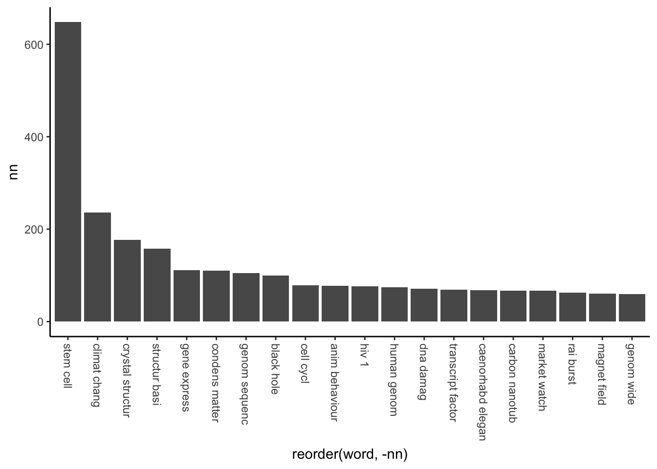
From this, it is very clear Nature’s main focus is on stem cells. The second place is climate change, but still ~2.75x less occurrence then the winner. “Crystal structure” and “structural basis” are mainly protein or polymer structures, which is a very popular field. If you are working in material science, better to go with these, or at least with carbon nanotubes
Condensed-matter physics is yet another article type, looks like we couldn’t clean all of them.
Gene expression, genome sequence/ing and cell cycle, DNA damage and transcription factor are the most popular molecular biology terms (of course after stem cell). If you want to publish a Nature paper, looks like these fields are the hot topics in life sciences.
If you are working in physics, probably black holes and magnetic fields are the best choices.
And the most popular biological model organism on full name: Caenorhabditis elegans with 68 occurrence in Nature article titles within 19 years. However Drosophila appeared 256 times. For a detailed look on the popularity of different model organisms, look at this table (human excluded, because it would take over everything):
Changing paradigms
So far so nice, I am already very glad with these results, but there are one more aspect I am interested. Research trends are changing in time, for example 19 years ago there was no genome sequencing, which take the place of genetic mapping.
bad_words <- c("scienc", "science", "review", "highlight", "research", "biology", "physics", "journal", "club", "communication", "al", "reply", "50", "100", "new")

all_words %>%
  mutate(year = lubridate::year(date)) %>%
  anti_join(stop_words, by = "word") %>%
  filter(!word %in% bad_words,
         year != 2017) %>%
  mutate(word = word %>% SnowballC::wordStem()) %>%
  group_by(year) %>%
  count(word, sort = TRUE) -> word_count_year

word_count_year
## Source: local data frame [76,318 x 3]
## Groups: year [19]
##
## # A tibble: 76,318 x 3
## year word nn
## <dbl> <chr> <int>
## 1 2009 cell 196
## 2 2008 cell 186
## 3 2006 cell 174
## 4 2005 cell 150
## 5 2013 cell 144
## 6 2014 cell 140
## 7 2007 cell 138
## 8 2015 cell 138
## 9 2004 cell 134
## 10 2001 cell 130
## # ... with 76,308 more rowsFirst of all let’s see the number of words in every year.
word_count_year %>%
  filter(year != 2017) %>%
  group_by(year) %>%
  summarize(sum = sum(nn)) %>%
  ggplot() +
  geom_line(aes(x = year,
                y = sum),
size =2) 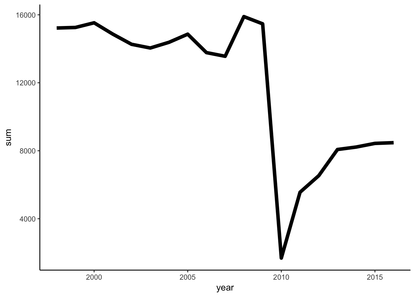
Look’s like in 2010 there was less publications or extra short titles. We can find out, if we just see the number of publications by year.
all_title %>%
  mutate(year = lubridate::year(date)) %>%
  filter(year != 2017) %>%
  group_by(year) %>%
  summarize(sum = value %>%
              length() %>%
              sum()) %>%
  ggplot() +
  geom_line(aes(x = year,
                y = sum),
            size = 2) +
  labs(title = "Number of Publications in Nature",
       x = "Year",
y = "Number of publications") 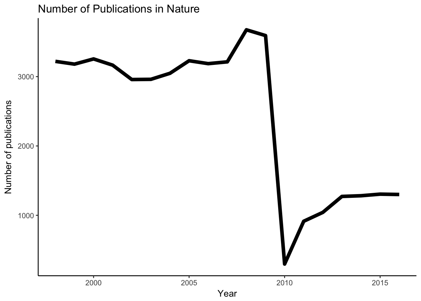
Looks like the publication number is radically dropped in 2010. I am not sure about the exact cause, but interestingly Nature Communications came out in that year in the first time also. Probably Nature decided to distribute the publications in several subjournals and keep just the top few in Nature itself.
full_join(
all_title %>%
  mutate(year = lubridate::year(date)) %>%
  filter(year != 2017) %>%
  group_by(year) %>%
  summarize(publication_sum = value %>%
              length() %>%
              sum()) ,
word_count_year %>%
  filter(year != 2017) %>%
  group_by(year) %>%
  summarize(word_sum = sum(nn)),
by = "year"
) %>%
  mutate(av_title_length = word_sum/publication_sum) %>%
  ggplot() +
  geom_line(aes(x = year,
                y = av_title_length),
            size = 1,
            color = "dodgerblue") +
  geom_point(aes(x = year,
                 y = av_title_length),
             color = "dodgerblue",
             size = 2) +
  geom_line(aes(x = year, y = word_sum/max(word_sum)* max(av_title_length)), color = "red", alpha = 0.3) +
  geom_line(aes(x = year, y = publication_sum/max(publication_sum)* max(av_title_length)), color = "green", alpha = 0.3) +
  labs(title = "Avarage Title Length in Nature",
       x = "Year",
       y = "Words in Title",
       caption = c("Red line: average word number in titles (relative)\nGreen line: Publication number in issues (relative)"))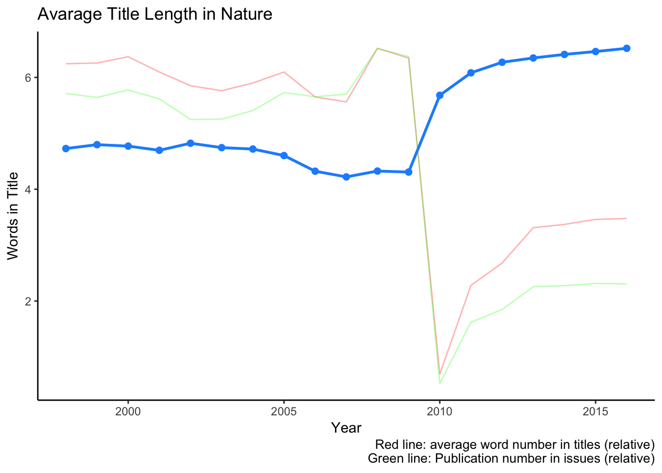
Fewer article number probably allowed slightly longer, better explanatory titles to articles. Other possibility is the increasing complexity of articles where finding an appropriate and short title is almost impossible.
Detailed search on specific terms
There is a lot more we could do in general, but then I would never finish this post. If you have any idea please comment below. If you put some R code, or result on your work and founding, that is the best.
Now let’s have a look in some specific terms. Here I will focus mainly on terms which are relevant to my field, molecular biology, genomics and evolution. Also I will look for some global events’ influence, like some disease outbreak. I put the R code for every post, but will not explain them, since they are repetitive and relatively easy to understand. If you have different interest, then me, please show your results and findings and let’s compare what happened in the scientific life in the point of view of Nature.
Publication influence from main disease outbreaks
Let’s have a look on major disease outbreaks from the past decades, like several flu types, Ebola and SARS.
word_count_year %>%
  filter(word %in% c("h1n1", "h5n1", "h7n9", "ebola", "sar")) %>%
  full_join(word_count_year %>%
           filter(year != 2017) %>%
           group_by(year) %>%
           summarize(word_sum = sum(nn)),
           by = "year") %>%
  filter(!is.na(nn)) %>%
  ggplot() +
  geom_line(aes(x = year,
                y = nn/word_sum,
                color = word),
            alpha = 0.6,
            size =1.5) +
  geom_point(aes(x = year,
                y = nn/word_sum,
                color = word),
            alpha = 0.9,
            size =2) +
  labs(x = "Year",
       y = "Relative abudance (%)",
       title = "Disease outbreaks") +
  scale_x_continuous(breaks = 1998:2016, limits = c(1998,2016)) +
  theme(panel.grid.major.x = element_line(color = "grey80"),
        axis.text.x = element_text(angle = 60, vjust = 0.5))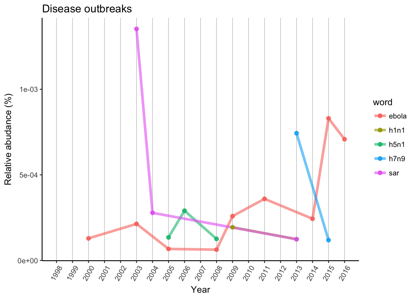
SARS was the first big outbreak from this plot, which started in 2002 November in South China and presented for almost 2 years with around 8000 cases. In 2003 there was a peak in publications, then in 2004 it was reported much less time and did not appeared again until 2013.
Ebola has a more constant base. It can be found in some African countries since 1995, but usually just a few hundred cases in a year. In 2013 there was a bigger outbreak in West Africa which was followed by a spread outside of Africa in 2014. Publication rate can give back this trend, with the peak in 2015, when scientists could react to the epidemic.
Influenza had several outbreaks with several strains. First H5N1 strain, which caused bird flu was discovered in 2004 and had publications in following years, 2005, 2006 and 2008. Swine flu (strain H1N1) was reported in 2009, and Nature had publication in the same year. FYI this is the same strain which caused Spanish flu in 1918. H7N9 strain of bird flu came in 2013, again the same year scientists reacted in Nature. There was recent outbreaks in 2016 October in China, so it is possible we can see similar trends in the future.
As conclusion we can say that scientists and Nature reacted to these outbreaks and recently with less time delay, which give some hope for faster and more effective vaccination and/or treatment development.
Appearance of genomics
Now let’s see a little more abstract scientific world and search for terms and techniques relevant to genomic research.
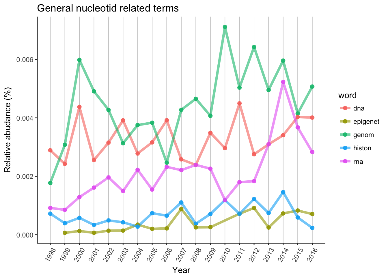
DNA and genome has similar patterns, however genome has 2 bigger peaks. One was possible the first genomes, human genome project and so. Later the popularity of new generation sequencing techniques allowed to sequence in way lower price then before, and the “genomic era” was started in mid-late 2000’. RNA is probably the newest and most popular big target to genetic/genomic research now. Histone and epigenetic related titles accumulating much slower, probably the real breakthrough is still waiting.
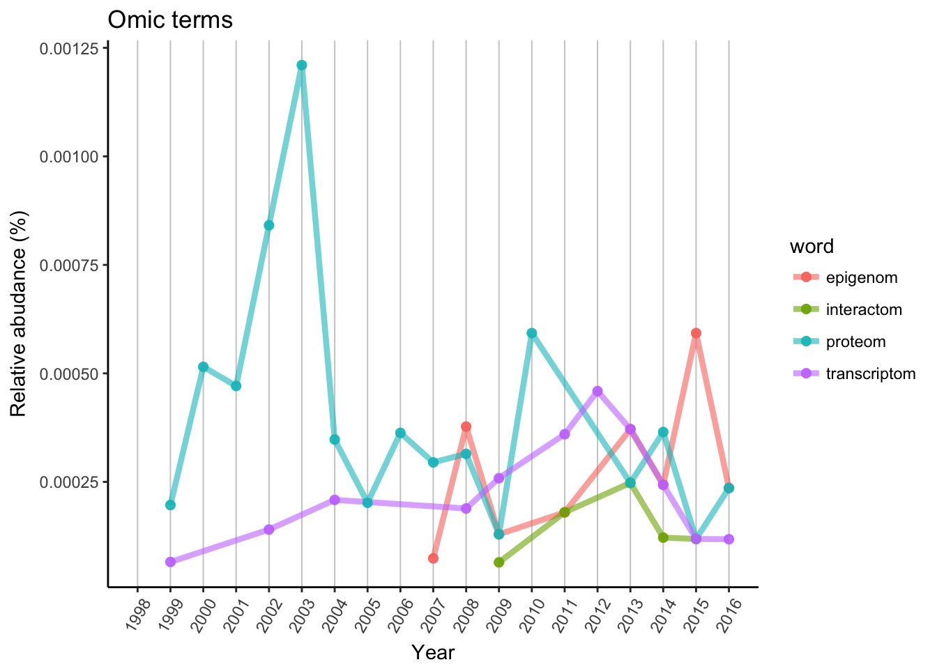
In early 2000’ proteomic research was on top due to MS/MS possibilities, but unfortunately there is no new or highly advanced technique, although there was several improvement. Transcriptomic research started slowly, and noways it cannot stand alone as a Nature paper. Epigenomic had a few peaks, but started relatively late, only appeared in 2007. Still 2 years earlier, then the first interactome paper. Interactome requires much higher amount of data and labor work, so the popularity is lower or similar then any other “omics” topic.
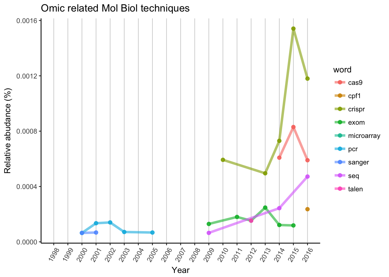
As we can expect, a single PCR or Sanger sequencing is not enough anymore to publish in Nature. Microarray is not represented, but “seq” can be found in rapidly increasing popularity, as in RNA-seq, ChIP-seq and so. Exom sequencing is also a great technique, but limitations of available organisms are stopped the wide spreading (mainly used for humans).
We can see the discovery and “incubation” of CRISPR, until researchers described the possible usage in genome editing. CRISPR/Cas9 is the first and most popular in use, but Cpf1 is also joined the race in 2016. Other genome editing methods are way underrepresented, as for TALEN system, there is only one data point in 2012.
Search for others
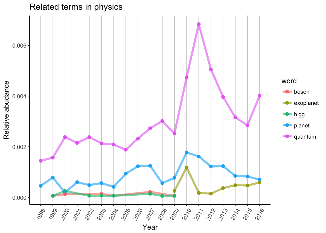
I am not familiar with the really hot topics in physics, just wanted to show You can search for anything which is interesting for You. Probably You can explain more about the events in Your field, then me. For example why the terms “Higgs” and “boson” disappeared in 2009? Why “exoplanet” appeared in the same year? What kind of exoplanet topic made the 2010 peak? What happened in quantum physics around 2011 and 2016?
If you have answers or made a small analysis on your own interest, found some other way to analyse or just have a question, please comment below. As an extra exercise, you can do similar analysis, but in different journals.